While taking Spacecraft Senior Design at Georgia Tech I and eight other team members had to design a spacecraft to land on Mars. All the high level analyses needed for an actual mission such science requirements, thermal and communication constraints and budget. Each major section was assigned to a team member, and I was designated to handle the trajectory analysis, which included both orbital analysis and Entry, Descent, and Landing (EDL). While most of the other groups in the class used simple equations for EDL, I decided to take it one step further and simulate the full 6 Degree of Freedom (6-DOF) Mars landing.

Lander

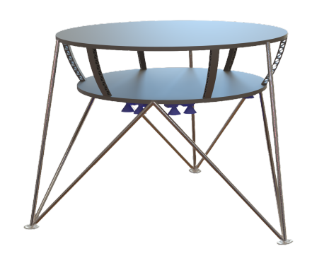
The lander for this mission is similar to the lander from the InSight mission. It uses heat shield and parachutes to slow itself down in the upper atmosphere and differential thrust to orient itself during the landing phase. Six thrusters are placed in around the hexagonal body and oriented in a way to give full controllability along roll, pitch and yaw. Below is an image of the lander with all the tanks and science experiments removed.

Optimal Control

In order to compute the trajectory of a mars lander we can reformulate the problem from a controls problem to a optimization problem. The problem becomes: given some initial and terminal conditions for what control input do I pick such that the mass is maximized at the final time given my dynamics. Below is a more mathematical description of the optimal control problem.

Section	Equation
Cost Function:	$\min_{t_f, \vec{u}} -m_f$
Initial Conditions:	$\vec{x}(0) = \vec{x}_0$
Terminal Conditions:	$\vec{x}(t_f) = \vec{x}_f$
Mass Dynamics:	$\dot{m} = -\frac{1}{I_{sp}g_0} \sum_{i=1}^{n_u} u_i$
Position Dynamics:	$\dot{\vec{r}} = \vec{v}$
Velocity Dynamics:	$\dot{\vec{v}} = \frac{1}{m} C_I^B \sum_{i=1}^{n_u} \hat{d}_i u_i + \vec{g}$
Quaternion Dynamics:	$\dot{\vec{q}} = \frac{1}{2} \Omega(\vec{\omega})\vec{q}$
Angular Velocity Dynamics:	$\dot{\vec{\omega}} = J_B^{-1}( \sum_{i=1}^{n_u} \vec{l}_i \times (\hat{d}_i u_i) - \vec{\omega} \times (J_B \vec{\omega}))$
Control Constraints:	$u_{\min} < u_i < u_{\max} \quad \forall i \in [1, n_u]$

Explanation of Variables

• $m$: Mass
• $t_f$: Final time
• $\vec{u}$: Control input vector (e.g., thrust)
• $\vec{x}$: State vector
• $I_{sp}$: Specific impulse
• $g_0$: Standard gravity
• $n_u$: Number of control inputs
• $\vec{r}$: Position vector
• $\vec{v}$: Velocity vector
• $C_I^B$: Direction Cosine Matrix (Inertial to Body frame)
• $\hat{d}_i$: Thrust direction unit vector for $i$-th thruster
• $\vec{g}$: Gravity vector
• $\vec{q}$: Quaternion (attitude representation)
• $\vec{\omega}$: Angular velocity vector
• $\Omega(\vec{\omega})$: Skew-symmetric matrix or equivalent operator for quaternion kinematics
• $J_B$: Inertia tensor (Body frame)
• $\vec{l}_i$: Lever arm vector for $i$-th thruster
• $u_{\min}, u_{\max}$: Minimum and maximum control limits

Most of the complexity of this optimization problem comes from the dynamics. Because this is a 6 Degree of Freedom simulation, we are taking into account the position and velocity as well as orientation and angular rate. Including mass, the total system the total system dynamics include 14 states (1 mass, 3 position, 3 velocity, 4 quaternion, and 3 angular rate). Below are some more details on exactly how the derivatives of the states are expressed.

Mass rate of change

$$\dot{m} = -\frac{1}{I_{sp}g_0} \sum_{i=1}^{n_u} u_i$$

This mass rate of change is a function of the thrust of each engine. The amount of thrust produced is proportional to the rate of change of the mass scaled by the specific impulse $I_{sp}$ and standard gravity $g_0$.

Position rate of change

$$\dot{\vec{r}} = \vec{v}$$

This is the most simple equation which simply relates that the time derivative of position in the inertial frame is the velocity in the inertial frame.

Linear Acceleration

$$\dot{\vec{v}} = \frac{1}{m} C_I^B \sum_{i=1}^{n_u} \hat{d}_i u_i + \vec{g}$$

The acceleration of the spacecraft is caused by the sum of forces of all the thrusters in the body frame which are then converted into the inertial frame with the rotation matrix $C^B_I$. This force is the divided by the mass and finally inertial gravity vector is then summed to the acceleration.

Quaternion rate of change

$$\dot{\vec{q}} = \frac{1}{2} \Omega(\vec{\omega})\vec{q}$$

This equation describes how the spacecraft’s orientation represented as a quaternion $q$ changes over time due to its angular velocity $\omega$. The matrix $\Omega(\omega)$ is a skew symmetric matrix which converts angular velocity into the rate of change of the quaternion.

Angular Acceleration

$$\dot{\vec{\omega}} = J_B^{-1}( \sum_{i=1}^{n_u} \vec{l}_i \times (\hat{d}_i u_i) - \vec{\omega} \times (J_B \vec{\omega}))$$

The angular acceleration of the spacecraft is defined by the moments produced by the thrusters by taking the cross product of the lever arm ($l_i$) with the thrust direction ($\hat{d}_i u_i$). A more simple version of the dynamics is shown below where $M_B$ is the moments in the body frame of the spacecraft.

$$\dot{\vec{\omega}} = J_B^{-1}( M_B - \vec{\omega} \times (J_B \vec{\omega}))$$

$$M_B=\sum_{i=1}^{n_u} \vec{l}_i \times (\hat{d}_i u_i)$$

A detailed formulation of these 6-DOF dynamics can be found in technical literature such as Basile Graf. “Quaternions And Dynamics”.

Successive Convexification (SCvx)

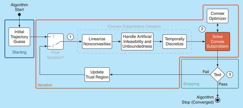
SCvx also known as Successive Convexification is a numerical algorithm to solve nonlinear optimal control problems. Direct non-linear optimization is difficult because of all the nonconvex dynamics and constraints. Gradient based solvers like IPOPT (Interior-point optimization) often get stuck for 6-DoF control problems like this one. The trick the SCvx solvers is to not solve the entire problem in one go but rather simplify the problem into a sequence of easier convex subproblems.

At each iteration the linear nonlinear dynamics and constraints are linearized around the trajectory leading to a optimization problem that is convex. Usually this problem is formulated as a Second-Order Cone Program (SOCP) which can be solved using solvers such as MOSEK. The resulting trajectory is then used as the new reference trajectory for the next iteration. This loop is repeated until the trajectory converges.

Below is a image from a paper titled “Convex Optimization for Trajectory Generation: A Tutorial on Generating Dynamically Feasible Trajectories Reliably and Efficiently,” that shows a high level diagram of how the algorithm works.

Problem Setup

The powered descent phase of a mars landing can be broken down in two different sections. The first is slowing the vehicle down and removing most of the kinetic energy. The next section is called Constant Velocity (CV). This is when the vehicle starts to hover close to the ground at a constant velocity. These two phases can be formulated each as it’s own optimization problem. Below are tables of the initial, intermediate (Start of CV) and terminal conditions.

State	Initial Conditions	Start of CV	Final Condition
Position (m)	$[0, 0, 900]$	$[50, 200, 8]$	$[50, 200, 0]$
Velocity (m/s)	$[0, 0, -59.7]$	$[0, 0, -1]$	$[0, 0, -1]$
Quaternion	$[1, 0, 0, 0]$	$[1, 0, 0, 0]$	$[1, 0, 0, 0]$
Angular Rate (rad/s)	$[0, 0, 0]$	$[0, 0, 0]$	$[0, 0, 0]$

Parameter	Value
$g_0 (\frac{m}{s^2})$	$9.81$
$I_{sp} (s)$	$225$
$J_b (kg \cdot m^2)$	$\text{diag}(81.5, 81.5, 163)$
$n_u$	$6$
$u_{min} (N)$	$31$
$u_{max} (N)$	$1200$

Results

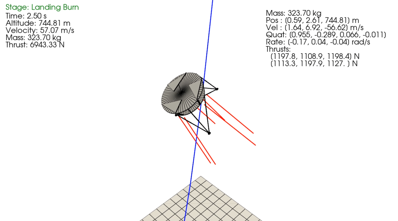
The animation below is a visual overview of the landing with the associated landing burn phase and constant velocity phase.

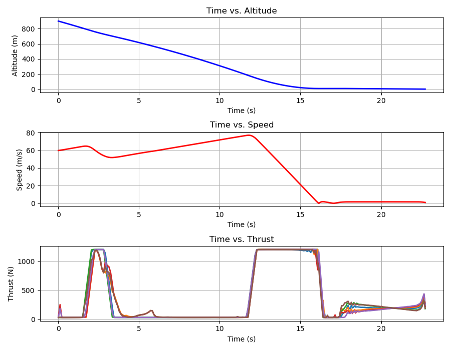
The figure above shows three different plots. The first plot shows the vehicle altitude as a function of time and the second plot shows vehicle speed as a function of time. The third plot is a bit more interesting, this shows the thrust of all the thrusters as a function of time. What is interesting is that the thrust control acts like a bang-bang controller, meaning the thrust is either at its maximum or minimum.

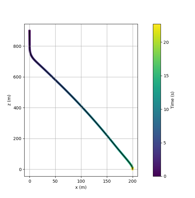
The second figure shows a 2D cross-section of the trajectory from initial conditions to terminal conditions.

Conclusion

Ultimately, this Senior Design experience proved that using high-fidelity dynamics with algorithms, such as SCvx can be used for precision-landing missions. This technical project helped me better understand optimal control theory and rigid body dynamics, which will strongly influence my future work in aerospace engineering.

Citations

[1] D. Malyuta, T. P. Reynolds, M. Szmuk, T. Lew, R. Bonalli, M. Pavone, and B. Açıkmeşe, “Convex Optimization for Trajectory Generation: A Tutorial on Generating Dynamically Feasible Trajectories Reliably and Efficiently,” IEEE Control Syst. Mag., vol. 42, no. 5, pp. 40–113, Oct. 2022, doi: 10.1109/MCS.2022.3187542.

[2] B. Graf, “Quaternions And Dynamics,” arXiv e-prints, Feb. 2007. Available: https://arxiv.org/pdf/0811.2889