Golf Ball UKF Tracker

software

By David Reynolds
December 27, 2023 - 6 min read

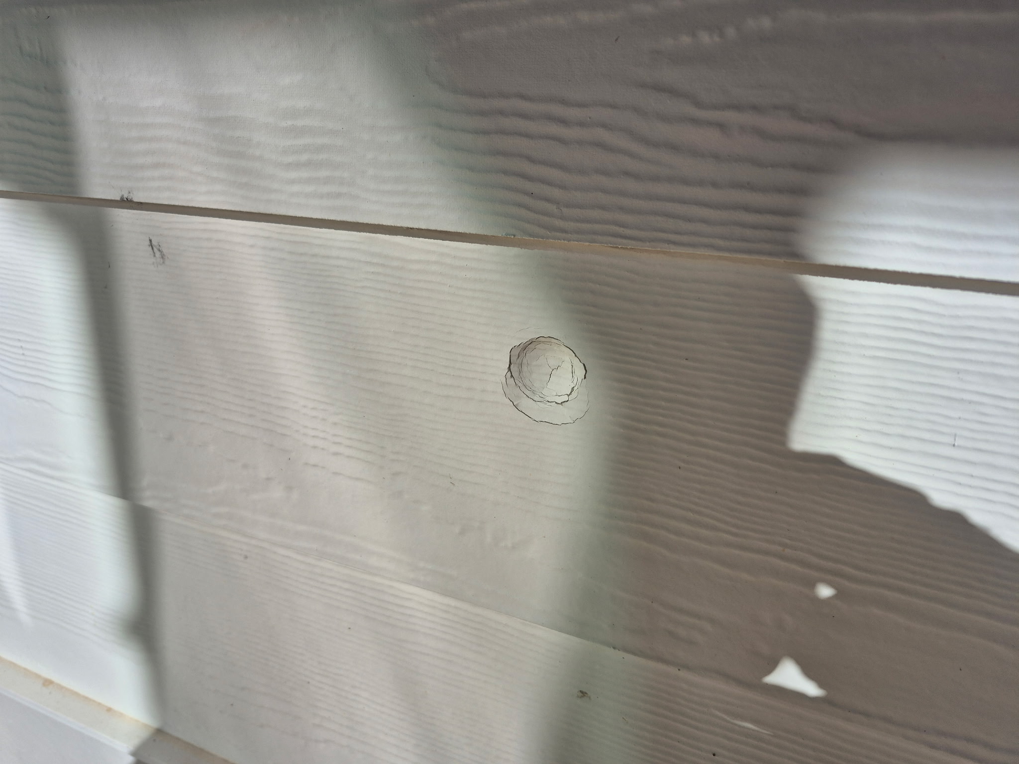
Recently, my parents moved into a beautiful new house directly on a golf course. This is heaven for my dad, who loves golf, but there is one major problem with living directly on a course: golf balls! Unfortunately, a few terrible golfers have already hit the house, as seen in the picture below.

Alt text

This got me thinking: what if I made my own Iron Dome system to defend the house against golf balls? There are two major parts to this problem: the first is tracking, and the second is interception. I focused my energy on the first problem of tracking and simulated it in MATLAB to see if it was possible.

Golf Ball Dynamics

Before we can track a golf ball we first must be able to simulate it as a dynamical system. Almost all dynamical systems can be written in the form of $\dot{\mathbf{x}}=f(\mathbf{x})$ and a golf ball is no exception. The state vector $\mathbf{x}$ holds position, velocity and angular rate totaling 9 states and 6 degrees of freedom.

$\mathbf{x} = \begin{bmatrix} \vec{x} \\ \vec{v} \\ \vec{\omega} \\ \end{bmatrix}$

where:

$\vec{x} = [x, y, z]^T$ is the position vector in the inertial frame
$\vec{v} = [v_x, v_y, v_z]^T$ is the velocity vector in the inertial frame
$\vec{\omega} = [\omega_x, \omega_y, \omega_z]^T$ is the angular rotation in the body frame

	Dynamics
Position Dynamics	$\dot{\vec{x}}=\vec{v}$
Velocity Dynamics	$\dot{\vec{v}}=\frac{1}{2m}\rho AC_D \|\vec{v}-\vec{w}\|(\vec{v}-\vec{w}) + \frac{1}{2m} \rho A C_L \|\vec{v}-\vec{w}\| \left(\frac{\vec{\omega} \times (\vec{v}-\vec{w})}{\|\vec{\omega}\|} \right) + \vec{g}$
Rotational Dynamics	$\dot{\vec{\omega}}=\tau \vec{\omega}$

The complexity of the trajectory arises from the velocity dynamics, which can be broken down into three major components:

The first is drag acceleration which comes from the standard drag formula of $\frac{1}{2m} \rho AC_D|\vec{v}-\vec{w}|(\vec{v}-\vec{w})$ with the velocity being subtracted by the current wind.
The second section is calculating lift caused by the magnus effect. If you ever wonder why golf balls curve or climb in the air, this is why. The rotational spin on the ball produces a lift effect which causes the golf ball to accelerate. The magnus acceleration is modeled as: $\frac{1}{2m}\rho A C_L |\vec{v}-\vec{w}|\left(\frac{\vec{\omega} \times (\vec{v}-\vec{w})}{|\vec{\omega}|} \right)$ . Looking at the formula the faster the ball spins the more lift the ball generates.
Finally the last part of the velocity dynamics is gravity which is a constant vector downward of -9.81 m/s.

For the Rotational dynamics the angular acceleration of the ball is modeled as a exponential decay with $\tau$ being a negative number $\dot{\vec{\omega}}=\tau \vec{\omega}$ .

These dynamics can be written in the form $\dot{\mathbf{x}}=f(\mathbf{x})$ which when combined with a ode solver can calculate the trajectory of the entire golf ball given some initial condition.

Camera Projection

In order to track the golf balls we need a sensor that can detect where the ball is. There are many sensors I could have picked but the one I used were simple optical cameras. The mathematical process to convert the position of the golf ball in global inertial frame to camera coordinates are as shown below where $R$ is a rotation matrix from local camera frame to the global frame and $b$ is the vector from the origin to the camera.

$P_{local} = R^T \cdot (P_{global}-b)$

Once the position of the golf ball is in the local camera frame it can then be converted to a $u$ and $v$ frame defined below.

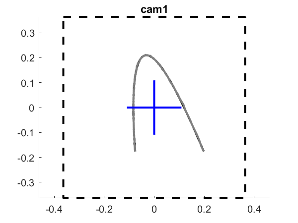
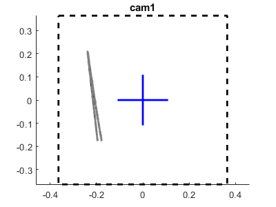
$\begin{aligned} u &= \frac{x}{y} \\ v &= \frac{z}{y} \end{aligned}$

Below is are some results on what the 3d trajectory of the golf ball looks like along side what the camera views.

Tracking (UKF)

Now that we have a way to simulate our sensor, we need to take those measurements and somehow determine our state (position, velocity, and spin). There are many ways to do this, but the most advanced and robust method is using a Kalman Filter. A Kalman Filter takes in noisy measurements and a system model to produce an optimal estimate of the current state, accounting for the uncertainty in both the dynamics and the measurements. Put simply, a Kalman Filter is a tracker—in this case, it’s tracking golf balls.

There are two ways to implement the Kalman Filter for nonlinear systems. The first is using an Extended Kalman Filter (EKF) and the other uses a unscented Kalman Filter (UKF). While there are several technical differences between the two, the UKF is often more efficient and easier to implement because it does not require calculating a Jacobian at every time step.

Every Kalman Filter works by maintaining a state estimate and using new measurements to update the uncertainty of that state. You can think of this uncertainty as a “confidence bubble” around the estimate. The UKF works by propagating a specific set of sigma points from this uncertainty distribution through the actual nonlinear dynamics. By observing where these points land, the filter can calculate a new, more accurate estimate and uncertainty. This process of calculating uncertainty by passing discrete points through a nonlinear function is known as the Unscented Transform.

UKF Initialization

The first step in the UKF is setting some tuning parameters. These parameters tell the UKF how to distribute the sigma points. Below is the formula for $\lambda$ which is the parameter for sigma point spacing.

$\lambda = \alpha^2 (N+\kappa)-N$

where

$\alpha$ is a tuning parameter from 0 to 1 which controls the spread of sigma points
$N$ is the number of states. In our example $N=9$
$\kappa$ is a secondary scaling parameter that is usually set to 0

From this the weighs for the sigma points can be computed using the formula below.

$\begin{aligned} w_0^{(m)} &= \lambda / (N + \kappa) \\ w_0^{(c)} &= \lambda / (N + \lambda) + (1 - \alpha^2) + \beta \\ w_i &= 1 / 2(N + \lambda), \quad i > 0 \end{aligned}$

where

$w_0^{(m)}$ is the weight of the first sigma point when computed around the mean
$w_0^{(c)}$ is the weight of the first sigma point when computed around the covariance
$w_i$ is the weight of the other sigma points when computed around the mean or covariance

Finally before the main algorithm can run the user must specify an initial state $\hat{\mathbf{x}}_{0,0}$ and uncertainty $\mathbf{P}_{0,0}$ . If the initial states is not known then it can be set to a guess state and the initial uncertainty can be set to be a large number.

UKF Predict

The first part of the predict step is to calculate the sigma points that will get passed into the dynamics.

$\begin{aligned} \mathcal{X}_{n,n}^{(0)} &= \hat{\mathbf{x}}_{n,n} \\ \mathcal{X}_{n,n}^{(i)} &= \hat{\mathbf{x}}_{n,n} + \left( \sqrt{(N + \lambda) \mathbf{P}_{n,n}} \right)_i, & i &= 1, \dots, N \\ \mathcal{X}_{n,n}^{(i+N)} &= \hat{\mathbf{x}}_{n,n} - \left( \sqrt{(N + \lambda) \mathbf{P}_{n,n}} \right)_{i}, & i &= N+1, \dots, 2N \end{aligned}$

Once the sigma points are found the can be passed into the dynamics and propagated using a ODE solver.

$\mathcal{X}_{n+1,n} = f(\mathcal{X}_{n,n})$

Next a new estimate can found by taking a weighted average of the sigma points and a new covariance can be found using the formula below.

$\begin{aligned} \widehat{\mathbf{x}}_{n+1,n} &= \sum_{i=0}^{2N} w_i \mathcal{X}_{n+1,n}^{(i)} \\ \mathbf{P}_{n+1,n} &= \sum_{i=0}^{2N} w_i \left( \mathcal{X}_{n+1,n}^{(i)} - \widehat{\mathbf{x}}_{n+1,n} \right) \left( \mathcal{X}_{n+1,n}^{(i)} - \widehat{\mathbf{x}}_{n+1,n} \right)^T + \mathbf{Q} \end{aligned}$

The added $\mathbf{Q}$ matrix is the process noise which is added to account for any unmodeled disturbances such as wind.

UKF Update

The next step of the UKF algorithm is called the update step. In this step we correct our estimate and uncertainty with a new measurement. The first part og the update step is to transform our sigma points from state space to measurement using a observation function $\mathbf{h}$ .

$\mathcal{Z}_{n} = \mathbf{h}\left(\mathcal{X}_{n, n-1}\right)$

This observation function is the same function we defined above in the Camera Projection section. All this function does is project points from the state space ($\mathbf{x}$) into the observation space ($\mathbf{z}$), where the observation space is defined by $u$ and $v$ coordinates.

$\overline{\mathbf{z}}_{n} = \sum_{i=0}^{2 N} w_{i} \mathcal{Z}_{n}^{(i)}$

From these propagated sigma points, we can calculate a predicted measurement using the weighted mean of the points in the measurement space. In other words, $\overline{\mathbf{z}}_{n}$ represents our “best guess” of what the sensor will see, given our current state estimate. Next, we calculate the innovation covariance, $\mathbf{P}_{z_{n}}$ , and the cross-covariance, $\mathbf{P}_{xz_{n}}$ , between the states and measurements. These are found using the formulas below, where $\mathbf{R}_{n}$ represents the sensor uncertainty (or measurement noise). These matrices are essential because they determine the Kalman Gain, which dictates how much we should adjust our state estimate based on the difference between the actual and predicted measurements.

$\begin{aligned} \mathbf{P}_{z_{n}} &= \sum_{i=0}^{2 N} w_{i}\left(\mathcal{Z}_{n}^{(i)}-\overline{\mathbf{z}}_{n}\right)\left(\mathcal{Z}_{n}^{(i)}-\overline{\mathbf{z}}_{n}\right)^{T}+\mathbf{R}_{n} \\ \mathbf{P}_{x z_{n}} &= \sum_{i=0}^{2 N} w_{i}\left(\mathcal{X}_{n, n-1}^{(i)}-\widehat{\mathbf{x}}_{n, n-1}\right)\left(\mathcal{Z}_{n}^{(i)}-\overline{\mathbf{z}}_{n}\right)^{T}\end{aligned}$

From this the kalman gain can be calculated using the formula below.

$\mathbf{K}_{n} = \mathbf{P}_{x z_{n}}\left(\mathbf{P}_{z_{n}}\right)^{-1}$

The next formulas update the state estimate given the previous estimate and the current measurement, where $\mathbf{z}_{n}$ is the measurement received from the sensor. The covariance is also updated using the previous covariance and the calculated Kalman gain.

$\begin{aligned} \widehat{\mathbf{x}}_{n, n} &= \widehat{\mathbf{x}}_{n, n-1}+\mathbf{K}_{n}\left(\mathbf{z}_{n}-\overline{\mathbf{z}}_{n}\right) \\ \mathbf{P}_{n, n} &= \mathbf{P}_{n-1, n}-\mathbf{K}_{n} \mathbf{P}_{z_{n}} \mathbf{K}_{n}^{T} \end{aligned}$

With the update step complete, the filter has officially ‘fused’ the new camera data with our physical model. This continuous loop of prediction and correction allows the system to maintain a lock on the golf ball even if the sensor noise is high or the trajectory is highly non-linear.

Results

The initial conditions for the golf ball in the simulation with $v_0=50$ m/s and $\alpha=40^\circ$. The standard deviation of the camera measurement is 0.03 leading to the $\mathbf{R}$ be a 2 by 2 matrix with diagonals values of $0.03^2$ and all the diagonals of the $\mathbf{Q}$ matrix are 0.01.

State	Initial Conditions
Position (m)	$[15, -200, 0]$
Velocity (m/s)	$[0, v_0 \text{cos}(\alpha), v_0 \text{sin}(\alpha)]$
Angular Rate (rad/s)	$[10, 30, 100]$

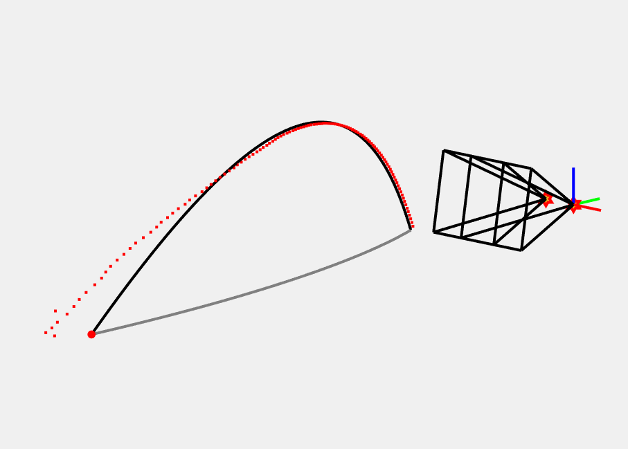
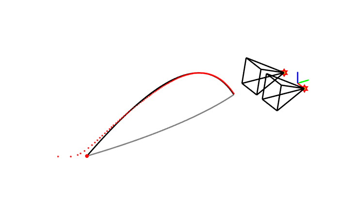
Below are some figures of trajectory with the black line representing the true value and the red dots representing the position estimate. The visualizations also include the camera frustums to show the sensors’ field of view, followed by the corresponding projected views from each camera.

Alt text

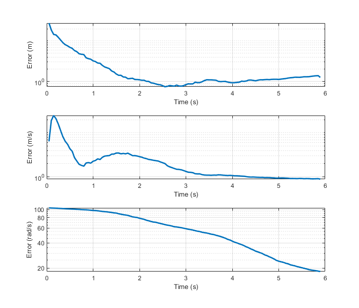
Below are the error plots, which shows a slow convergence over the flight. This trend indicates that as the sensors collect more data over time, the filter’s estimate becomes increasingly accurate, resulting in a steady reduction of error.

Alt text

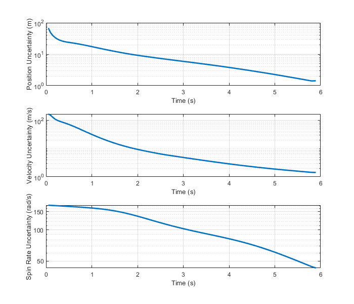
The same can be said for covariance which as shown below constantly decreases as time goes on.

Alt text

Monte Carlo

Because random noise is injected into the simulation to mimic real-life sensor behavior, every simulation run will be different. To fully evaluate the filter’s performance, a Monte Carlo simulation must be conducted. This is essentially a way of running the simulation many times to calculate the average performance of the filter across a wide range of random scenarios. Below is a figure of one such Monte Carlo plotting position error and uncertainty.

Alt text

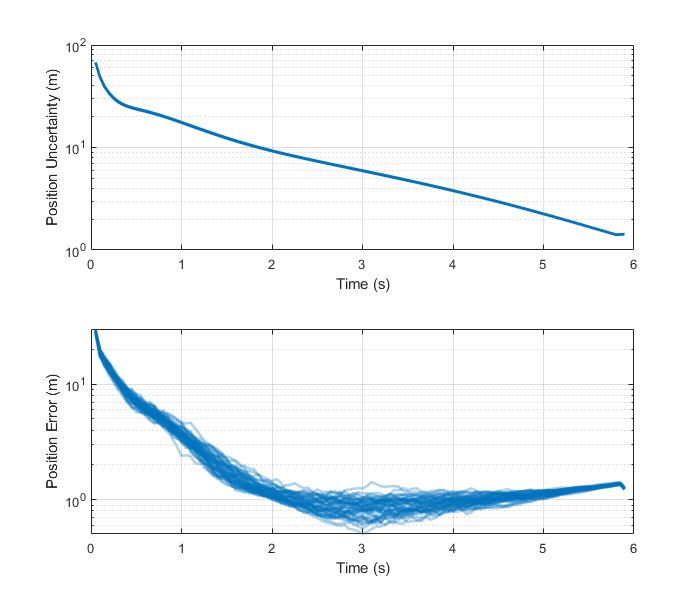
As one can see from the figure uncertainty does not change much from run to run. This is because at every run the same initial uncertainty and all the measurements are being pulled from the same distribution. The error bounces around much more as some runs get more lucky than others however, the Monte Carlo analysis shows that across hundreds of trials, the error consistently remains within our predicted “confidence bubble”.

Conclusion

So, what did all this math tell us? Well, first of all, the tracking problem is quite difficult. In our simulation, the sensor is very noisy; however, even when I turn the noise down, the uncertainty remains around 1 meter. I might be able to reduce this with more precise tuning, but the main point is that golf balls only have a radius of about 2 cm. This means I would need to reduce the uncertainty by almost two orders of magnitude to achieve a direct hit. This realization made it clear that a interception is a massive challenge, and for now, the most practical solution is to focus on a early warning system. While my house might still take a hit, at least we’ll see it coming.