Starship Control with LQR

tech

By David Reynolds
December 27, 2025 - 6 min read

Starship is one of the most interesting aerospace vehicles in existence. It is slated as the rocket that will send humanity to Mars, however I find it interesting for another reason, the controls. Looking at the Starship it does not have wings like a plane rather it has flaps and flies like a skydiver. This unconventional “belly flop” maneuver has left many wondering—how do you actually control such a vehicle?

To answer that question for myself, I took on the challenge of developing a full 6 Degree of Freedom (6-DOF) simulation. Building a high-fidelity model was the only way to truly capture the nuances of Starship’s flight. However, the simulation is only as good as the physics behind it, and the first major problem I encountered was getting an accurate aerodynamic model for such a complex shape. Luckily Peter Sharpe did this exact thing for his PhD during his time at MIT. He created something called the Aerosandbox which uses a neural net (Neuralfoil) to estimate aerodynamics coefficients for a given wing or fuselage at any orientation. The full library did way more but that is what I used it for, I encourage you to check it out.

https://github.com/peterdsharpe/AeroSandbox

The physics

Almost all dynamical systems can be written in the form of $\dot{\mathbf{x}}=f(\mathbf{x},\mathbf{u},t)$ and Starship is no exception. This formula is saying that the derivative of the state vector $\dot{\mathbf{x}}$ is a function of the current state $\mathbf{x}$, our control $\mathbf{u}$ and time $t$.

The state vector is all the necessary information to describe the state of the system. For this simulation, the state vector includes position in the inertial frame, velocity in the body frame, quaternion from inertial to body, and angular rate expressed in the body frame.

$\mathbf{x} = \begin{bmatrix} p_I \\ v_B \\ q_{IB} \\ \omega_B \end{bmatrix}$

where:

$p_I = [x, y, z]^T$ is the position vector in the inertial frame.
$v_B = [u, v, w]^T$ is the velocity vector in the body frame.
$q_{IB} = [q_0, q_1, q_2, q_3]^T$ is the quaternion representing the orientation from the inertial frame to the body frame.
$\omega = [\omega_x, \omega_y, \omega_z]^T$ is the angular velocity vector in the body frame.

The dynamics for starship (and any rigid body) are defined below

$\dot{p}_I=\mathbf{C}_{BI}v_B$

$\dot{v}_B = \frac{F_b}{m} + \mathbf{C}_{IB}(q) g$

$\dot{q} = \frac{1}{2} \boldsymbol{\Omega}(\omega) q$

$\dot{\omega} = \mathbf{I}_b^{-1} \left(M_b - \omega \times (\mathbf{I}_b \omega) \right)$

where:

$F_b$ is the sum of external forces in the body frame.
$M_b$ is the sum of external moments (torques) in the body frame.
$g = [0, 0, -9.81]^T$ is the gravitational acceleration vector in the inertial frame.
${C}_{IB}$ is the direction cosine matrix that transforms vectors from the inertial frame to the body frame (it is the transpose of ${C}_{BI}$ ). ${C}_{BI}={C}_{IB}^T$

$C_{IB}(q) = \begin{bmatrix} 1 - 2(q_2^2 + q_3^2) & 2(q_1 q_2 + q_0 q_3) & 2(q_1 q_3 - q_0 q_2) \\ 2(q_1 q_2 - q_0 q_3) & 1 - 2(q_1^2 + q_3^2) & 2(q_2 q_3 + q_0 q_1) \\ 2(q_1 q_3 + q_0 q_2) & 2(q_2 q_3 - q_0 q_1) & 1 - 2(q_1^2 + q_2^2) \end{bmatrix}$

$\mathbf{I}_b$ is the moment of inertia tensor in the body frame. Note that if the moment of inertia is dependent on the mass and CG location.
$\boldsymbol{\Omega}(w)$ is the skew-symmetric matrix representation of the angular velocity $\omega$.

$\boldsymbol{\Omega}(q) = \begin{bmatrix} 0 & -\omega_x & -\omega_y & -\omega_z \\ \omega_x & 0 & \omega_z & -\omega_y \\ \omega_y & -\omega_z & 0 & \omega_x \\ \omega_z & \omega_y & -\omega_x & 0 \end{bmatrix}$

If some of the math is a bit overwhelming then don’t worry. All you need to know is that the state vector holds the data on position, velocity, orientation, and angular rate and all the fancy equations tell us how those states change given some external forces and moments.

But where do those forces come from? In a vacuum, dynamics are simple, but Starship is flying through an atmosphere. Instead of blasting you with Greek letters, here is an intuitive way to think about the aerodynamics.

Every aerodynamic component such as a wing or a fuselage has aerodynamic properties such as lift, coefficient or drag coefficient. These properties when combined with speed and density can give a force and a moment. The total forces and moments acting on the Starship are found by summing the contributions of each individual component, including the secondary moments generated by forces acting away from the center of mass.

Pitch Control

In order to control the system we must linearize the dynamics around an operating point and apply linear control, however how are we supposed to do that when Starship is falling at terminal velocity? The trick is that we don’t linearize around the full 13 dimensional state vector. Rather we linearize around a reduced order model that only captures that thing we want to control, in this case pitch. So the state vector for pitch is as shown below. Where $x_4$ is a 4 dimensional state vector and $x_{13}$ is the full 13 dimensional state vector.

$\mathbf{x_4} = \begin{bmatrix} u \\ w \\ q \\ \theta \end{bmatrix}$

where:

$u$ is the x velocity in the body frame
$w$ is the z velocity in the body frame
$q$ is pitch rate
$\theta$ is pitch

If we can find a point in state space where $\mathbf{\dot{x}_4}$ is zero then we will have what is called a trim point. The full optimization formulation is shown below.

$$ \min_z || \frac{\partial g}{\partial x_4} f(\bar{x}(z), \bar{u}(z) ) ||^2 $$

In the formula $f$ is our dynamics defined above, $g$ is a function that takes in the full state vector and outputs the reduced state vector $x_4 = g(x_{13})$. The variables being optimized are $z$ which in this case are forward velocity ($u$) downward velocity ($w$) and pitch control. In order to convert pitch command to flap deflections an allocation matrix is used which is defined below.

$\begin{bmatrix} \delta_{fr} \\ \delta_{fl} \\ \delta_{br} \\ \delta_{bl} \end{bmatrix} = \begin{bmatrix} 1 & 1 & -1 & 1 \\ 1 & -1 & 1 & 1 \\ -1 & -1 & 1 & 1 \\ -1 & -1 & -1 & 1 \end{bmatrix} \begin{bmatrix} u_{pitch} \\ u_{yaw} \\ u_{roll} \\ u_{drag} \end{bmatrix}$

Once a trim point is found the dynamics can be linearized around that point by calculating the Jacobian of the dynamics with respect to the state and control and the trim point. The Jacobian can be calculated symbolically or using finite difference.

$A=\frac{\partial f}{\partial x}\Big\vert_{x=x^*} \qquad B=\frac{\partial f}{\partial u}\Big\vert_{u=u^*}$

From the linearization a LTI system can be derived as the following where $\delta_x=x-x^*$ and $\delta_u=u-u^*$ where $x$ is the reduced state vector of length 4.

$$ \delta \dot{x} = A \delta x+ B \delta u $$

From this we can use linear control techniques such as a Linear Quadratic Regulator (LQR). This control techniques works by minimizing the cost of a quadratic performance index subject to linear dynamics. The cost formulation is shown below where $Q$ is are the cost on the states and $R$ is the cost on the control. In our case $Q$ is a 4 by 4 matrix and $R$ is a scalar because we only have one control.

$$ J = \int_{0}^{\infty} (x^T Q x + u^T R u) dt $$

The control law that this formulation produces is in the form of a linear feedback law in the form $u=-Kx$. Because we are linearizing around a trim point the true control law is $u=-K \delta x$ where the delta is the change from the trim point.

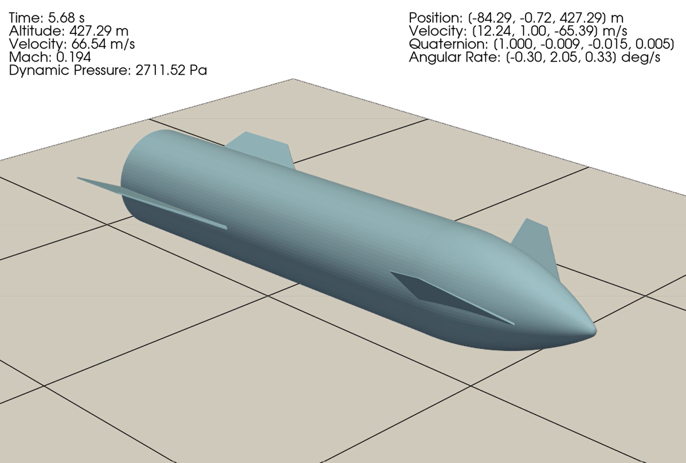
Results

Below is an animation of the controller working with added disturbances. In the animation below, I have introduced stochastic disturbances modeled as external moments. These are designed to simulate the sudden, unpredictable forces of wind shear that Starship would encounter during its long descent through the troposphere.

Alt text

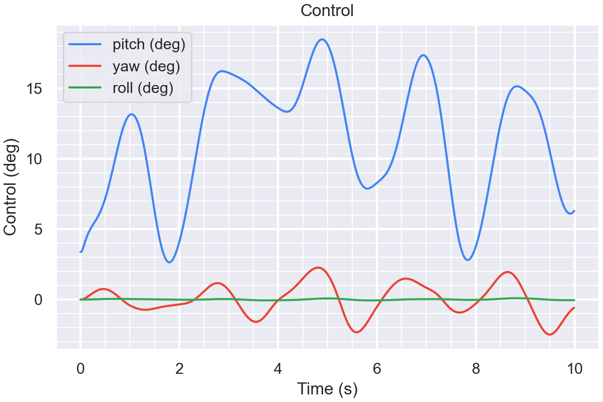
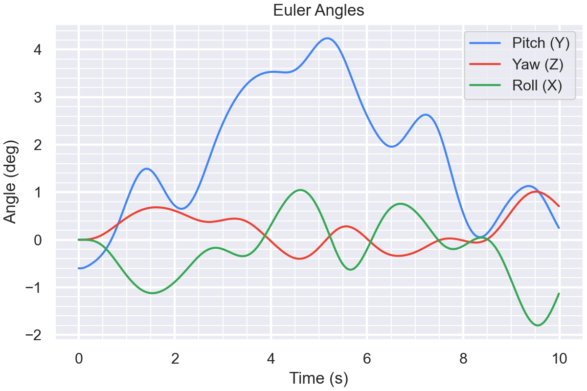
As one can see the pitch and yaw controllers are working to keep starship in its proper orientation.

Roadmap

While achieving a stable 6-DOF descent is a major milestone, the simulation is far from finished. To bring this project closer to the high-stakes reality of a SpaceX mission, I’ve outlined several key upgrades:

State Estimation (Kalman Filtering)
Monte Carlo analysis for robustness testing
Hypersonic reentry modeling
The iconic landing flip maneuver